Unlock the power of VLOOKUP in Excel with our comprehensive guide by Joboskill. Learn how to efficiently retrieve data, use syntax, and explore practical examples through video for better data management. Perfect for enhancing your Excel skills!
Microsoft Excel is a powerhouse of a spreadsheet program, packed with numerous functions to make data manipulation and analysis a breeze. One such function that stands out for its versatility and usefulness is VLOOKUP. Whether you’re a seasoned Excel user or just starting your spreadsheet journey, understanding and mastering the VLOOKUP function can significantly enhance your data-handling capabilities.
What is VLOOKUP?
VLOOKUP, which stands for Vertical Lookup, is a powerful function in Excel designed to search for a specific value in the first column of a table or range and return a corresponding value from another column. This function is particularly handy when you’re dealing with large datasets and need to quickly retrieve information based on specific criteria.
The Anatomy of VLOOKUP
Before diving into practical examples, let’s break down the syntax of the VLOOKUP function:
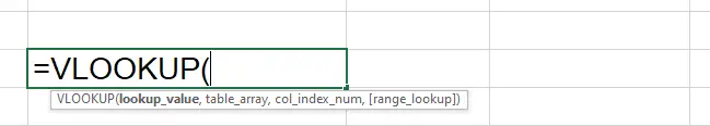
=VLOOKUP(lookup_value, table_array, col_index_num, [range_lookup])
- lookup_value: This is the value you want to search for in the first column of the table.
- table_array: This is the range of cells that contains the data. The first column of this range is where Excel will search for the lookup value.
- col_index_num: This is the column number in the table from which to retrieve the value. The first column in the table is 1, the second is 2, and so on.
- range_lookup: This is an optional argument. If set to TRUE (or omitted), Excel will look for an approximate match. If set to FALSE, it will look for an exact match.
Practical Examples
Example 1: Basic VLOOKUP
Let’s say you have a list of products in column A and their corresponding prices in column B. You want to find the price of a specific product. The formula would look like this:
=VLOOKUP("Product A", A1:B10, 2, FALSE)
This formula searches for “Product A” in the first column (A1 to A10) and returns the corresponding price from the second column (B1 to B10).
Example 2: Approximate Match
Imagine you have a table of grades and corresponding grade boundaries. You want to find the grade for a score. In this case, you might use an approximate match:
=VLOOKUP(85, A1:B6, 2, TRUE)
Here, Excel will find the closest match for the score 85 in the first column (A1 to A6) and return the corresponding grade from the second column (B1 to B6).
Tips for Success
- Ensure the Data is Sorted: For approximate matches, make sure the data in the first column of your table is sorted in ascending order.
- Handle Errors Gracefully: If the lookup value is not found, Excel returns an error. Use functions like IFERROR to display a custom message instead.
- Use Named Ranges: Instead of referencing cell ranges directly, consider naming your ranges. This makes your formulas more readable and easier to maintain.
- Combine with Other Functions: VLOOKUP works seamlessly with other Excel functions. For example, you can use it within an IF statement to perform more complex logic.
In conclusion, the VLOOKUP function in Excel is a valuable tool for efficiently retrieving information from large datasets. Mastering its usage can save you time and streamline your data analysis tasks. Experiment with different scenarios and embrace the power of VLOOKUP in your spreadsheet adventures!